Regression
For this lab, let’s use county-level 2020 presidential election results.
. * Set your working directory to the location of pres_county2020.dta
. use pres_county2020.dta, clear
Simple and Multiple Regression
. * SYNTAX: reg y x
. reg trump20pct trumppct

Source |       SS           df       MS      Number of obs   =     3,112
-------------+----------------------------------   F(1, 3110)      =  73277.15
Model |   775987.71         1   775987.71   Prob > F        =    0.0000
Residual |  32934.1652     3,110  10.5897637   R-squared       =    0.9593
-------------+----------------------------------   Adj R-squared   =    0.9593
Total |  808921.875     3,111  260.019889   Root MSE        =    3.2542

------------------------------------------------------------------------------
trump20pct |      Coef.   Std. Err.      t    P>|t|     [95% Conf. Interval]
-------------+----------------------------------------------------------------
trumppct |   .9776738   .0036117   270.70   0.000     .9705923    .9847554
_cons |  -.0372979   .2477361    -0.15   0.880    -.5230407    .4484449
------------------------------------------------------------------------------

.
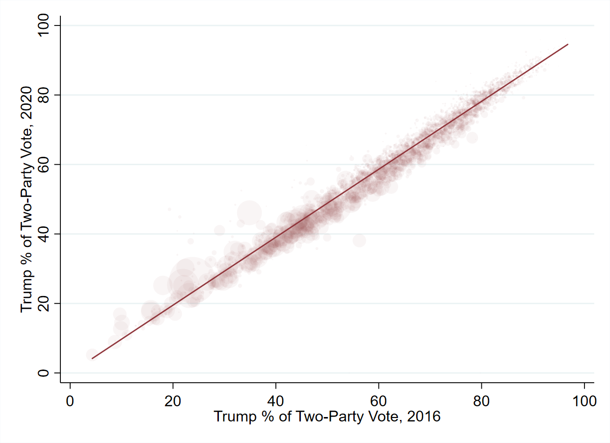
. * let's visualize:
. scatter trump20pct trumppct [pw=total20votes], ///
>     msize(small) mcolor(maroon%5) mlwidth(none) ///
>     graphregion(color(white)) ///
>     || lfit trump20pct trumppct, lcolor(maroon) ///
>      legend(off) xtitle("Trump % of Two-Party Vote, 2016") ///
>     ytitle("Trump % of Two-Party Vote, 2020")
 Now let’s conduct a multiple regression, adding county race and education variables:
. * SYNTAX: reg y x1 x2...
. reg trump20pct trumppct whitenoncollege whitecollege black latinx

Source |       SS           df       MS      Number of obs   =     3,111
-------------+----------------------------------   F(5, 3105)      =  20398.24
Model |  781995.993         5  156399.199   Prob > F        =    0.0000
Residual |  23806.9313     3,105  7.66728866   R-squared       =    0.9705
-------------+----------------------------------   Adj R-squared   =    0.9704
Total |  805802.924     3,110  259.100619   Root MSE        =     2.769

---------------------------------------------------------------------------------
trump20pct |      Coef.   Std. Err.      t    P>|t|     [95% Conf. Interval]
----------------+----------------------------------------------------------------
trumppct |   .9396296    .004703   199.79   0.000     .9304082     .948851
whitenoncollege |   7.180532   .8133951     8.83   0.000     5.585685    8.775379
whitecollege |  -13.35032   .9881584   -13.51   0.000    -15.28783   -11.41281
black |   4.517834   .8052197     5.61   0.000     2.939017    6.096651
latinx |   10.53558   .8616352    12.23   0.000     8.846147    12.22501
_cons |  -.6150971   .7359075    -0.84   0.403    -2.058012    .8278176
---------------------------------------------------------------------------------
Predictions and Residuals
Stata has built-in postestimation commands which help you extract additional information from your model results. predict is a very useful postestimation command, available for a wide range of model types, including OLS. We can use predict to calculated $$ as well as residuals ($y_i - $). predict will call up your most recent model results to use for analysis, or you could store your regression results and then call up whichever model results you want.
. quietly reg trump20pct trumppct

. * save regression results and name them "m1"
. estimates store m1

.
. quietly reg  trump20pct trumppct whitenoncollege whitecollege black latinx

. * save regression results and name them "m2"
. estimates store m2

.
. * now restore m1 results
. estimates restore m1
(results m1 are active now)

.
. *predict y_hat:
. * SYNTAX: predict newvar, options
. predict y_hat_m1
(option xb assumed; fitted values)
(107 missing values generated)

.
. *we could calculate residuals directly as well:
. predict residual_m1, residuals
(149 missing values generated)

.
. estimates restore m2
(results m2 are active now)

. predict y_hat_m2
(option xb assumed; fitted values)
(147 missing values generated)

. predict residual_m2, residuals
(150 missing values generated)
How well do our models match the actual Trump % in 2020? We could plot the predict values against our original DV:
. scatter trump20pct y_hat_m1, msize(vsmall) mcolor(maroon%15)
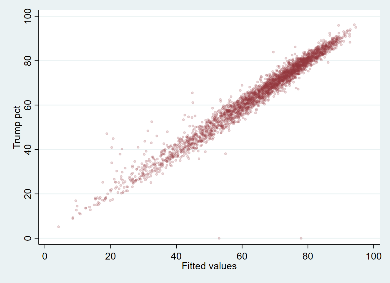 Pretty well!
. scatter trump20pct y_hat_m2, msize(vsmall) mcolor(maroon%15)
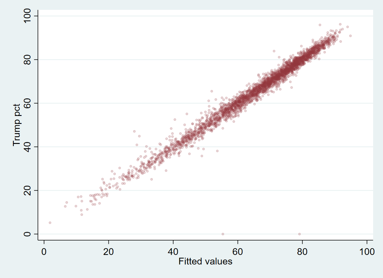
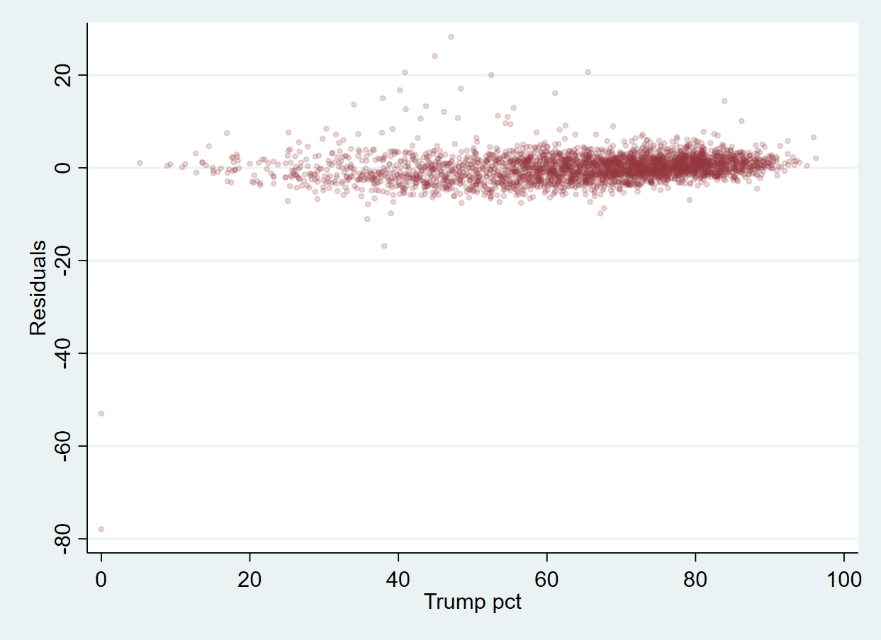
Even better, we can plot the residuals directly:
. scatter residual_m1 trump20pct , msize(vsmall) mcolor(maroon%15)
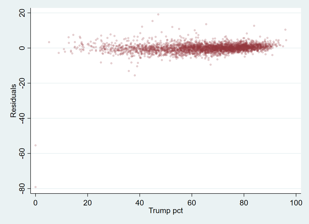
 And again:
. scatter residual_m2 trump20pct, msize(vsmall) mcolor(maroon%15)
Regression with nominal data
To incorporate independent variables measured at the categorical/nominal level, you need to create a series of dummy (dichotomous) variables. You could do so by hand using the recode command, or you could use Stata’s factor variable notation: add an i. in front of the variable name. An additional strategy is to use tab with the gen() option. I use strategies two and three in the example below.
. * add region dummies to the regression model
.
. *first create the dummies:
. tab region, gen(regdum)

region |      Freq.     Percent        Cum.
------------+-----------------------------------
1 |        217        7.01        7.01
2 |      1,056       34.10       41.10
3 |      1,366       44.11       85.21
4 |        458       14.79      100.00
------------+-----------------------------------
Total |      3,097      100.00

. describe regdum*

storage   display    value
variable name   type    format     label      variable label
--------------------------------------------------------------------------------------------------------------------------------------------------------------------------------------------------------
regdum1         byte    %8.0g                 region== 1.0000
regdum2         byte    %8.0g                 region== 2.0000
regdum3         byte    %8.0g                 region== 3.0000
regdum4         byte    %8.0g                 region== 4.0000

.
. *now run the regression, being sure to leave out one dummy (in this case, the South)
. reg trump20pct trumppct whitenoncollege whitecollege black latinx regdum1 regdum2 regdum4

Source |       SS           df       MS      Number of obs   =     3,055
-------------+----------------------------------   F(8, 3046)      =  13200.57
Model |  772218.983         8  96527.3729   Prob > F        =    0.0000
Residual |  22273.4542     3,046  7.31236185   R-squared       =    0.9720
-------------+----------------------------------   Adj R-squared   =    0.9719
Total |  794492.437     3,054  260.148146   Root MSE        =    2.7041

---------------------------------------------------------------------------------
trump20pct |      Coef.   Std. Err.      t    P>|t|     [95% Conf. Interval]
----------------+----------------------------------------------------------------
trumppct |   .9302781     .00513   181.34   0.000     .9202195    .9403367
whitenoncollege |   6.080273    .820377     7.41   0.000     4.471724    7.688821
whitecollege |  -14.28692   .9763185   -14.63   0.000    -16.20123   -12.37261
black |   .9215254   .8427074     1.09   0.274    -.7308073    2.573858
latinx |   9.670075   .8456495    11.44   0.000     8.011973    11.32818
regdum1 |  -.1633985   .2292055    -0.71   0.476    -.6128117    .2860147
regdum2 |  -.6834723   .1389635    -4.92   0.000     -.955944   -.4110006
regdum4 |  -2.318332   .1741424   -13.31   0.000    -2.659781   -1.976884
_cons |   1.814021   .7460239     2.43   0.015     .3512594    3.276782
---------------------------------------------------------------------------------

. estimates store m3

.
. *we could do a similar regression with i.region, but we won't be able to define
. * the reference category - Stata will the first category as the reference.
. reg trump20pct trumppct whitenoncollege whitecollege black latinx i.region

Source |       SS           df       MS      Number of obs   =     3,055
-------------+----------------------------------   F(8, 3046)      =  13200.57
Model |  772218.983         8  96527.3729   Prob > F        =    0.0000
Residual |  22273.4542     3,046  7.31236185   R-squared       =    0.9720
-------------+----------------------------------   Adj R-squared   =    0.9719
Total |  794492.437     3,054  260.148146   Root MSE        =    2.7041

---------------------------------------------------------------------------------
trump20pct |      Coef.   Std. Err.      t    P>|t|     [95% Conf. Interval]
----------------+----------------------------------------------------------------
trumppct |   .9302781     .00513   181.34   0.000     .9202195    .9403367
whitenoncollege |   6.080273    .820377     7.41   0.000     4.471724    7.688821
whitecollege |  -14.28692   .9763185   -14.63   0.000    -16.20123   -12.37261
black |   .9215254   .8427074     1.09   0.274    -.7308073    2.573858
latinx |   9.670075   .8456495    11.44   0.000     8.011973    11.32818
|
region |
2  |  -.5200738   .2103211    -2.47   0.013    -.9324594   -.1076882
3  |   .1633985   .2292055     0.71   0.476    -.2860147    .6128117
4  |  -2.154934    .237672    -9.07   0.000    -2.620947    -1.68892
|
_cons |   1.650622   .7534941     2.19   0.029     .1732137    3.128031
---------------------------------------------------------------------------------
Interaction terms and marginal effects
The easiest way to incorporate interaction terms into your regression analysis is by using Stata’s built-in interaction notation. ## signifies an interaction between two independent variables and will incorporate the interaction term into the model. For example: reg y c.x##c.z, assuming you want to treat x and z as ordinal or interval data, will include the constituent terms of x and of z along with the interaction xz. If x is nominal, you’d use: i.x instead of c.x.
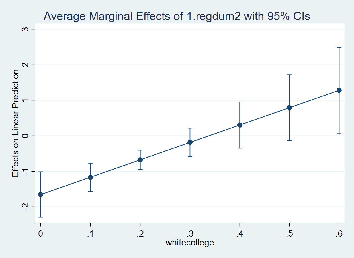
The margins command lets you calculate the predicted effect of your constituent variables AND their interaction on the dependent variable. We call these conditional marginal effects the effect of one variable, conditional on the other variable’s values (because of the interaction term, the predicted effect of x varies by z).
. reg trump20pct trumppct whitenoncollege black latinx regdum1 i.regdum2##c.whitecollege regdum4

Source |       SS           df       MS      Number of obs   =     3,055
-------------+----------------------------------   F(9, 3045)      =  11772.68
Model |  772297.501         9  85810.8334   Prob > F        =    0.0000
Residual |  22194.9365     3,045   7.2889775   R-squared       =    0.9721
-------------+----------------------------------   Adj R-squared   =    0.9720
Total |  794492.437     3,054  260.148146   Root MSE        =    2.6998

----------------------------------------------------------------------------------------
trump20pct |      Coef.   Std. Err.      t    P>|t|     [95% Conf. Interval]
-----------------------+----------------------------------------------------------------
trumppct |   .9291103   .0051341   180.97   0.000     .9190436     .939177
whitenoncollege |   6.034341   .8191837     7.37   0.000     4.428132     7.64055
black |   .5535949   .8487943     0.65   0.514    -1.110673    2.217863
latinx |   9.384419   .8487705    11.06   0.000     7.720198    11.04864
regdum1 |  -.0818514   .2301836    -0.36   0.722    -.5331824    .3694796
1.regdum2 |  -1.652678   .3262698    -5.07   0.000    -2.292409   -1.012947
whitecollege |  -15.77708   1.075309   -14.67   0.000    -17.88549   -13.66867
|
regdum2#c.whitecollege |
1  |   4.885712   1.488598     3.28   0.001     1.966954     7.80447
|
regdum4 |  -2.275541   .1743519   -13.05   0.000    -2.617401   -1.933682
_cons |    2.23724   .7559097     2.96   0.003     .7550952    3.719385
----------------------------------------------------------------------------------------

. estimates store m4

. * the dydx(regdum2) option requests Stata calculate the marginal effect of being in the Midwest
. * over the values specified in the at() command, in this case, when whitecollege moves from 0
. * to .6 in units of .1.
. margins, dydx(regdum2) at(whitecollege=(0(.1).6))

Average marginal effects                        Number of obs     =      3,055
Model VCE    : OLS

Expression   : Linear prediction, predict()
dy/dx w.r.t. : 1.regdum2

1._at        : whitecollege    =           0

2._at        : whitecollege    =          .1

3._at        : whitecollege    =          .2

4._at        : whitecollege    =          .3

5._at        : whitecollege    =          .4

6._at        : whitecollege    =          .5

7._at        : whitecollege    =          .6

------------------------------------------------------------------------------
|            Delta-method
|      dy/dx   Std. Err.      t    P>|t|     [95% Conf. Interval]
-------------+----------------------------------------------------------------
0.regdum2    |  (base outcome)
-------------+----------------------------------------------------------------
1.regdum2    |
_at |
1  |  -1.652678   .3262698    -5.07   0.000    -2.292409   -1.012947
2  |  -1.164107   .2017281    -5.77   0.000    -1.559644   -.7685696
3  |  -.6755355   .1387622    -4.87   0.000    -.9476125   -.4034584
4  |  -.1869643    .205266    -0.91   0.362    -.5894382    .2155097
5  |   .3016069   .3306536     0.91   0.362    -.3467199    .9499337
6  |    .790178   .4699446     1.68   0.093    -.1312627    1.711619
7  |   1.278749   .6137447     2.08   0.037     .0753535    2.482145
------------------------------------------------------------------------------
Note: dy/dx for factor levels is the discrete change from the base level.

.
. * marginsplot will graph the results from the margins command. Check out help marginsplot to
. *  see some of the options you can use to change the look of the graph.
. marginsplot

Variables that uniquely identify margins: whitecollege
Presentation of Results
My favorite ways of presenting regression results require adding user-generated Stata commands. You can add such commands from Boston College’s Statistical Software Components (SSC) archive through ssc install. We’ll use two packages: estout and coefplot.
esttab
The esttab command, from the estout package, is, in my opinion, the best way to generate regression tables in Stata. The command lets you make tables of multiple regression models, gives you flexibility over which parameter estimates to include, and formatting control over the look of the table.
. * install the estout package from the SSC
. ssc install estout
checking estout consistency and verifying not already installed...
all files already exist and are up to date.

.
. * SYNTAX: esttab model_names, options
. *   the m1 through m4 item below are our stored model names from previous regressions
. *   b se options tell Stata to include the coefficients (b) and standard errors (se)
. *   star() option lists a symbol and then the significance level
. *   the wide option places standard errors to the right of coefficients instead of
. *      underneath the coefficients - good if you have multiple models to include
. *      in the table.
. *   the ar2 option adds the Adj. R^2 score at the bottom of the table.
.
. esttab m1 m2 m3 m4, b se star(+ .1 * .05 ** .01) wide ar2

----------------------------------------------------------------------------------------------------------------------------
(1)                         (2)                         (3)                         (4)
trump20pct                  trump20pct                  trump20pct                  trump20pct
----------------------------------------------------------------------------------------------------------------------------
trumppct            0.978**    (0.00361)        0.940**    (0.00470)        0.930**    (0.00513)        0.929**    (0.00513)
whitenonco~e                                    7.181**      (0.813)        6.080**      (0.820)        6.034**      (0.819)
whitecollege                                   -13.35**      (0.988)       -14.29**      (0.976)       -15.78**      (1.075)
black                                           4.518**      (0.805)        0.922        (0.843)        0.554        (0.849)
latinx                                          10.54**      (0.862)        9.670**      (0.846)        9.384**      (0.849)
regdum1                                                                    -0.163        (0.229)      -0.0819        (0.230)
regdum2                                                                    -0.683**      (0.139)
regdum4                                                                    -2.318**      (0.174)       -2.276**      (0.174)
0.regdum2                                                                                                   0            (.)
1.regdum2                                                                                              -1.653**      (0.326)
0.regdum2#~e                                                                                                0            (.)
1.regdum2#~e                                                                                            4.886**      (1.489)
_cons             -0.0373        (0.248)       -0.615        (0.736)        1.814*       (0.746)        2.237**      (0.756)
----------------------------------------------------------------------------------------------------------------------------
N                    3112                        3111                        3055                        3055
adj. R-sq           0.959                       0.970                       0.972                       0.972
----------------------------------------------------------------------------------------------------------------------------
Standard errors in parentheses
+ p<.1, * p<.05, ** p<.01

.
. * You can save the table directly to your computer!
. quietly esttab m1 m2 m3 m4 using regmodels.csv, b se star(+ .1 * .05 ** .01) wide r2 csv replace
coefplot
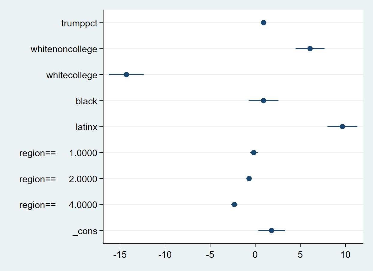
The coefplot command offers an easy way to graph coefficient estimates and confidence intervals around those estimates. coefplot works best when your variables are the same.
. * install the coefplot package
.
. ssc install coefplot
checking coefplot consistency and verifying not already installed...
all files already exist and are up to date.

.
. * load the m3 model results
. estimates restore m3
(results m3 are active now)

.
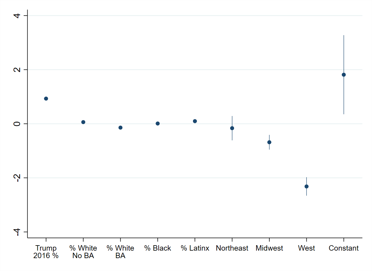
. coefplot
 Let’s switch to vertical orientation:
. * now let's make the dots vertical:
. coefplot, vertical
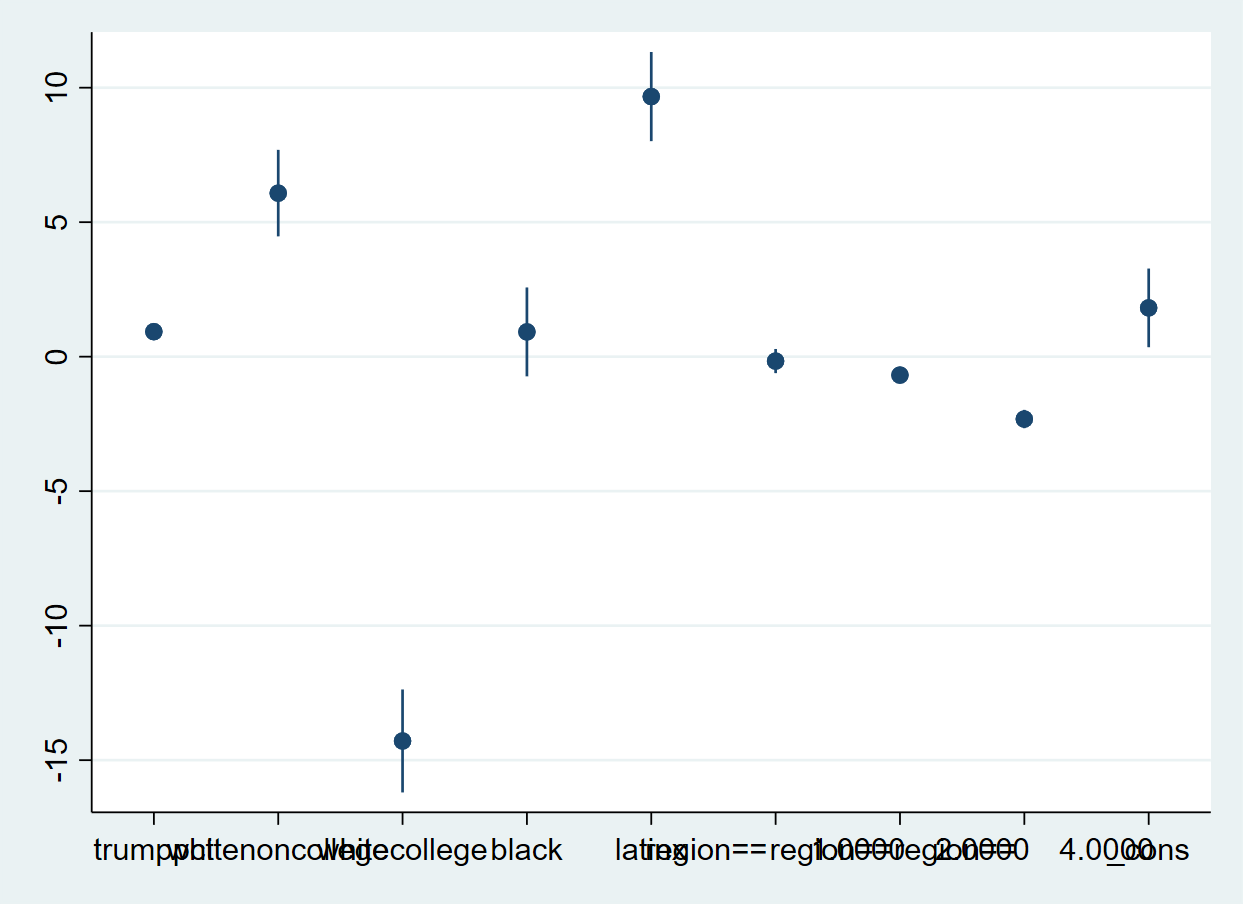 And clean up the graph to make it easier to read:
.
. * let's rescale our proportion variables and change the labels, marker size, and graph color:
. coefplot, vertical msize(small) ciopts(lwidth(vthin)) rescale(whitenoncollege = .01 whitecollege = .01 black = .01 latinx = .01) ///
>     coeflabels(trumppct = `""Trump""2016 %""' whitenoncollege = `""% White""No BA""' whitecollege = `""% White""BA""' ///
>     black = "% Black" latinx = "% Latinx" regdum1 = "Northeast" regdum2 = "Midwest" regdum4 = "West" ///
>     _cons = "Constant" , labsize(small)) graphregion(color(white))
